I’m assuming you understand the basic idea of neural networks. This essay focuses purely on the backpropagation algorithm itself.
What is Backpropagation?
Backpropagation is an algorithm that computes how much each weight and bias should change to reduce the loss.
It tells us not just whether parameters should go up or down, but by how much, based on their actual impact on the loss function. We use math to figure out that.
The Key Players
Before we dive in, let’s identify what we’re working with:
- Input data - what we feed into the network
- Parameters - weights (w) and biases (b) that we need to adjust
- Neurons - the computational units
- Loss - measures how wrong our predictions are
- Target - what we’re trying to predict
What is a Neuron?
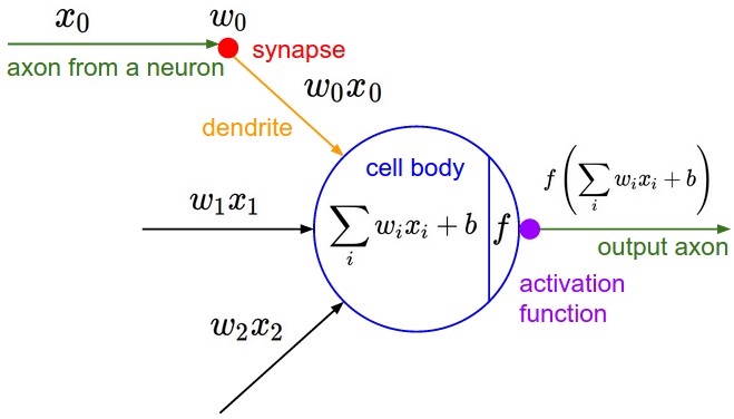 A neuron performs two simple computations:
z = w · a + b
a_out = σ(z)
Where:
- a is the input activation (from the previous layer)
- w is the weight
- b is the bias
- z is the weighted sum (pre-activation) -> z = sum((wi) x (xi)) + b
- σ is the activation function (sigmoid, ReLU, etc.)
- a_out is the output activation
Think of it like this: the neuron takes inputs, weighs them, adds a bias, then applies a non-linear function. That’s it.
The Forward Pass
Training involves:
- Forward pass - feed input through the network to get a prediction
- Compute loss - measure how wrong the prediction is
- Backward pass - figure out how to adjust weights to reduce loss
- Update weights - make the adjustments
- Repeat
The forward pass is straightforward. The backward pass is where backpropagation comes in.
The Goal: Minimize Loss
We want to reduce the loss. The tool we use is gradient descent.
Why gradient descent?
Gradients tell us about the movement of some function(in our case the loss function) wrt some variable (in our case, the parameters).
Gradient descent is the idea that we try to move in the opposite direction to the gradient vector to minimize the cost function.
Why opposite direction? Because gradient vector points to the direction of steepest increase.
Gradient Descent Intuition
Imagine you’re blindfolded on a hilly terrain trying to reach the lowest valley.
What would you do?
- Feel the slope under your feet
- Determine which direction goes downhill most steeply
- Take a small step in that direction
- Repeat
In mathematical terms:
- The terrain = Loss function (how wrong your model is)
- Your position = Current parameter values
- Feeling the slope = Computing the gradient ∂L/∂w
- Taking a step = Updating: w ← w - η · ∂L/∂w
The gradient ∂L/∂w tells us which direction is “downhill” for the loss.
The Problem: We Can’t Compute ∂L/∂w Directly
Here’s the issue: the loss doesn’t directly depend on w. What do I mean? Suppose there are 2 million layers.
the 101th layer’s third neuron. Think about that neuron. We want to figure out the Loss’s derivative wrt to THAT neuron. They are just too far away from each other.
The dependency chain looks like this:
w → z → a → (more layers) → prediction → loss
The loss is computed way at the end, but w is buried deep in the network. They’re connected through many ==intermediate computations==.
This is why we need the chain rule.
The Chain Rule Solution
To compute ∂L/∂w, we break it into pieces:
∂L/∂w = ∂L/∂a · ∂a/∂z · ∂z/∂w
Let’s understand each term:
∂z/∂w - “How does z change when w changes?” Looking at z = w·a + b, we get: ∂z/∂w = a This is local and easy to compute.
∂a/∂z - “How does activation change when z changes?”
This depends on the activation function:
- Sigmoid: σ’(z) = σ(z)(1 - σ(z))
- ReLU: σ’(z) = 1 if z > 0, else 0
This is also local and easy.
∂L/∂a - “How does loss change when this activation changes?” This is the tricky one. And this is where the interaction between layers happen! For hidden layers, we don’t know this directly. We have to get it from the layer ahead.
The Backpropagation Algorithm
Backpropagation works backwards through the network:
Step 1: Output Layer (Easy Case)
At the output layer, ∂L/∂a can be computed directly from the loss function.
For example, if Loss = (prediction - target)², then:
∂L/∂a^L = 2(a^L - target)
Step 2: Compute Local Gradients
For each neuron at this layer:
- Compute ∂a/∂z = σ’(z)
- Compute ∂z/∂w = a (the input to this neuron)
Step 3: Multiply Using Chain Rule
∂L/∂w = ∂L/∂a · ∂a/∂z · ∂z/∂w
Now we have the gradient for this weight!
Step 4: Pass Gradients Backward
For the previous layer to compute its gradients, it needs ∂L/∂a.
We compute it using:
∂L/∂a^prev = w · ∂L/∂z
Where ∂L/∂z = ∂L/∂a · ∂a/∂z (combining the first two terms).
Step 5: Repeat
Move to the previous layer and repeat steps 2-4, using the ∂L/∂a we just computed.
Continue until you’ve computed gradients for all weights in all layers.
The Complete Picture
Forward pass: Input → Layer 1 → Layer 2 → … → Output → Loss
Backward pass: Loss → ∂L/∂w_output → ∂L/∂w_layer2 → … → ∂L/∂w_input
Each layer:
- Receives ∂L/∂a from the next layer
- Computes its own ∂L/∂w using the chain rule
- Passes ∂L/∂a_prev to the previous layer
Update the Weights
Once we have ∂L/∂w for every weight:
w ← w - η · ∂L/∂w
b ← b - η · ∂L/∂b
This nudges each parameter in the direction that reduces loss.
Implementation Note: PyTorch
While trying to implement a Tensor class myself, I got to know that each tensor holds the dL/d(that tensor w) in the .grad attribute.
x = torch.tensor(2.0, requires_grad=True)
y = x * 3
y.backward()
print(x.grad)
one shot
Backpropagation is elegant:
- Do a forward pass and compute loss
- Start at the output where ∂L/∂a is known
- Use the chain rule to compute ∂L/∂w locally
- Pass ∂L/∂a backwards to the previous layer
- Repeat until all gradients are computed
- Update all weights using gradient descent
The “back” in backpropagation refers to this backward flow of gradients through the network, from output to input. This algorithm is also ‘greedy’.
Neural Net
We now know that a neural network is simply a set of parameters optimized to minimize a loss function. A good exercise to internalize this idea is the following.
You are given the XOR problem:
// XOR problem.
// X -> inputs, y -> true values
float X[4][2] = {{0,0}, {0,1}, {1,0}, {1,1}};
float y[4][1] = {{0}, {1}, {1}, {0}};

// Random weights and biases.
float w1[2][2];
float b1[2][1];
float w2[2][1];
float b2[1][1];
Writing backpropagation for this problem is what helped me develop an intuitive understanding of how backpropagation works. The task is simple: after training, the loss function (which can be any reasonable choice) should be minimized, meaning the forward pass produces accurate outputs for the XOR problem.
For the sake of simplicity, here is a simple solution in python
import numpy as np

def loss(yt, y):
    return np.mean((yt - y) ** 2)

X = np.array([[0,0],[0,1],[1,0],[1,1]])
y = np.array([[0],[1],[1],[0]])  # XOR

W1 = np.random.randn(2,2)
b1 = np.zeros((1,2))
W2 = np.random.randn(2,1)
b2 = np.zeros((1,1))
lr = 0.1

print("Initial weights and biases:")
print(f"W1:\n{W1}\nb1:\n{b1}\nW2:\n{W2}\nb2:\n{b2}")
print("*" * 60)

for epoch in range(5000):
    # Feedforward
    z1 = X @ W1 + b1
    a1 = sigmoid(z1)
    z2 = a1 @ W2 + b2
    y_hat = sigmoid(z2)

    # Calculate loss
    epoch_loss = loss(y_hat, y)

    # Backprop
    dz2 = y_hat - y
    dW2 = a1.T @ dz2
    db2 = np.mean(dz2, axis=0, keepdims=True)

    dz1 = (dz2 @ W2.T) * sigmoid_prime(z1)
    dW1 = X.T @ dz1
    db1 = np.mean(dz1, axis=0, keepdims=True)

    # Update weights
    W1 -= lr * dW1
    b1 -= lr * db1
    W2 -= lr * dW2
    b2 -= lr * db2

    if epoch % 1000 == 0:
        print(f"Epoch {epoch}: Loss = {epoch_loss:.6f}")

# Activation function
def sigmoid(z):
    return 1 / (1 + np.exp(-z))

def sigmoid_prime(z):
    return sigmoid(z) * (1 - sigmoid(z))
print("\n" + "=" * 60)
print("Final predictions:")
print("y_hat", y_hat)
for i in range(len(X)):
    print(f"Input: {X[i]} -> Predicted: {y_hat[i][0]:.4f}, Actual: {y[i][0]}")
Thanks for reading
~ Aayushya Tiwari
REFERENCES
Watch the Andrej Karpathy Micrograd Video for super intuition. Or 3b1b’s video. They are the best.
NN in NUMPY book pdf: my first reference to backprop
Original paper