Today we’re looking at LSTM (Long Short Term Memory) neural networks.

The standard for sequential data was RNNs (Recurrent Neural Networks).
RNNs had an issue. They were good at remembering things, but they… well, they kept forgetting too!
They had what we call a vanishing gradient problem.

Small example to guide your visual senses:

The spine of the problem is, when the gradients flow backwards, they get multiplied. And say if that number that we’re multiplying with is smaller - which a lot of times the gradients are, then at some point the gradient will be close to zero and boom you’ve lost signal.
At each timestep, the gradient gets multiplied by the derivative of the activation function (like sigmoid) — a number that maxes out at 0.25. Ten steps back, your gradient is 0.25¹⁰ — essentially zero.

LSTMs fix this by changing the math from multiplication to addition. In a vanilla RNN, the gradient is forced through a “squashy” activation function at every single step, which rapidly shrinks it.

The LSTM’s “secret sauce” is that the cell state update is additive ($c_t = c_{prev} \cdot f + ...$). If the forget gate is “open” (close to 1), the gradient can flow backwards through this additive “spine” across hundreds of timesteps almost unchanged. This is often called the Constant Error Carousel, and it’s what finally allows the “Long” part of Long Short Term Memory to actually work.

LSTM

LSTMs introduced a cell state. The vanilla RNN had a h_t which had two jobs: be the “memory passed forward” and “output signal”.
But when we overwrite the h_t, we lost the signal from 10 units ago.

LSTM’s cell state is an additional state that is only changed when the gates have to change it. And $h_t$ here now remains the output signal.

Now the math is pretty simple. It is essentially 4 equations, which we will also implement in code.

Input gate: $i = \sigma(x \cdot W_i + b_i)$

Forget gate: $f = \sigma(x \cdot W_f + b_f)$

Candidate: $\tilde{c} = \tanh(x \cdot W_c + b_c)$

Output gate: $o = \sigma(x \cdot W_o + b_o)$

Cell state: $c_t = c_{prev} \cdot f + \tilde{c} \cdot i$

Hidden state: $h_t = o \cdot \tanh(c_t)$

The first four define the gates. The last two are what actually happens to the state.

The Input gate is the entry point of data to the network. We do a simple linear operation with $W_i$ (weights of input gate) and addition with $b_i$ (bias of input gate), applying an activation function after it.

The Forget gate is what data the network wants to forget at the current timestep. The Candidate is what data the network wants to learn. We use both of these in the cell state.

For the gates we use sigmoid to squash to (0, 1) — a valve. For the candidate we use tanh to squash to (-1, 1) — a value with direction.

code

import torch
import torch.nn as nn

class LSTM(nn.Module):

    def __init__(self, input_size, hidden_size):
        # input : [batch, input_size + hidden_size]
        super().__init__() # [batch size, hidden + input]
        self.w_i = nn.Parameter(torch.randn([input_size + hidden_size, hidden_size])) # input
        self.w_f = nn.Parameter(torch.randn([input_size + hidden_size, hidden_size])) # forget 
        self.w_c = nn.Parameter(torch.randn([input_size + hidden_size, hidden_size])) # candidate 
        self.w_o = nn.Parameter(torch.randn([input_size + hidden_size, hidden_size])) # output gate

        self.bi = nn.Parameter(torch.zeros([hidden_size, ]))
        self.bf = nn.Parameter(torch.zeros([hidden_size, ]))
        self.bc = nn.Parameter(torch.zeros([hidden_size, ]))
        self.bo = nn.Parameter(torch.zeros([hidden_size, ]))

    def forward(self, x, h_prev, c_prev): # at each timestep
        '''
        at each timestep: we have two things, x and h_prev. We concat them and say that use this curr input and also the previous hidden states
        to make decisions and do calculations.  
        '''
        x = torch.cat([h_prev, x], dim=1) # raw tensors, we're adding previous hidden states. 

        i = torch.sigmoid(x @ self.w_i + self.bi) # pass through input gate
        f = torch.sigmoid(x @ self.w_f + self.bf) # pass through forget gate
        c_curr = torch.tanh( x @ self.w_c + self.bc) # memory state
        o = torch.sigmoid(x @ self.w_o + self.bo) # output gate

        c_t = c_prev * f + c_curr * i 
        h_t = o * torch.tanh(c_t)

        return c_t, h_t

In init we define four weight matrices and four biases — one per gate, plus the candidate. In forward, the first thing we do is concatenate h_prev and x into a single vector. From that point on, every gate sees both the current input and the previous hidden state in one shot. After the six calculations, we return c_t and h_t — the updated memory and the output signal.

x = torch.cat([h_prev, x], dim=1)

The concatenation happens because we want the gates to take as input both the previous hidden state and the current input as learning data.

training a model

input dataset:

df = sns.load_dataset('flights')

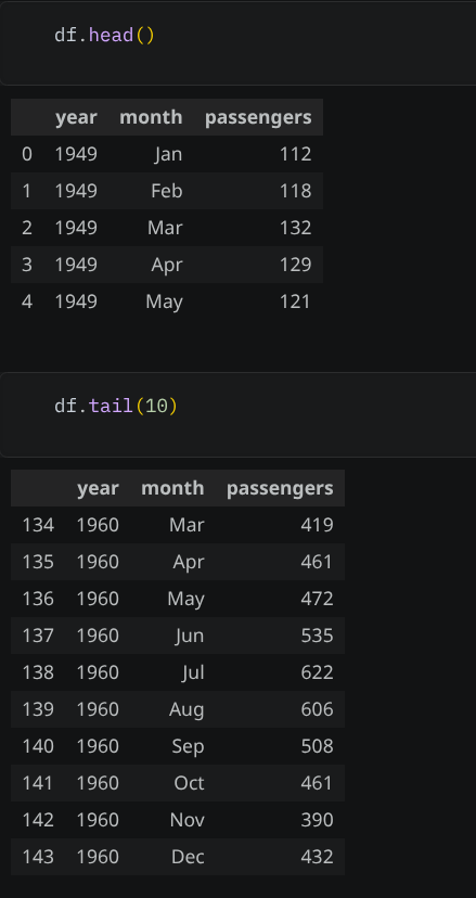
The dataset contains the number of passengers month-wise from 1949 to 1960.
We preprocess the dataset such that the problem becomes:

given 12 months previous data, predict this month’s number of passengers

X = torch.tensor(X).unsqueeze(-1) # 132, 12, 1
y = torch.tensor(y)
print(X.shape)
print(y.shape)

>>torch.Size([132, 12, 1])
>>torch.Size([132])

We now initialize the model, optimizer and loss_function

lstm = LSTM(input_size=1, hidden_size=32)
linear = nn.Linear(32, 1)

optimizer = torch.optim.Adam(list(lstm.parameters()) + list(linear.parameters()), lr=0.01)
loss_fn = nn.MSELoss()

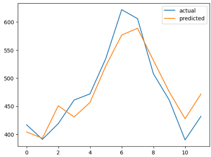So our training was successful. We got 0.0713 loss after 200 epochs.

This was an article on LSTM.

Thanks for reading
~ Aayushya

LSTM#

code#

training a model#

LSTM

code

training a model