My final year project is Chase-the-cloud: Cloud motion prediction using INSAT 3DR data. And, it’s been some time since I’ve sat down to write about what I have been working on. And to be fair, this project has made me question my life’s existence more than any other project, like ever.
So, let’s talk about it.
To make you interested in what we’re going to be talking about, here’s a picture of a trained model’s prediction:
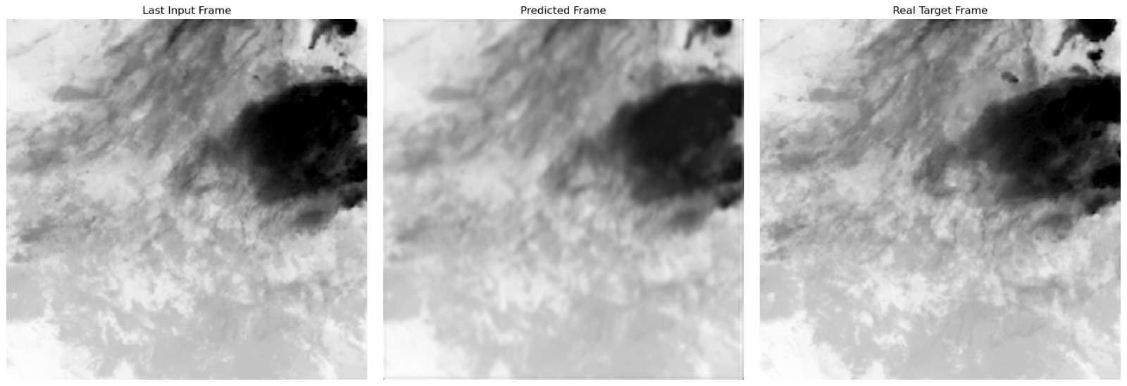
Left is the last frame, middle is the prediction, right is the real target frame. We will talk about it in details later in this piece.
what is the project?
The project formally:
We formulate future-frame generation as a spatiotemporal prediction problem, where a model is given a sequence of $K$ past frames, $X_{t-K+1}, \ldots, X_t$, and learns to predict the subsequent frame $\hat{X}_{t+1}$. Formally, the model learns a function $f_\theta$ such that $\hat{X}_{t+1} = f_\theta(X_{t-K+1}, \ldots, X_t)$, capturing both the spatial structure within individual frames and the temporal dynamics across frames. The model is trained by minimizing a loss $\mathcal{L}(\hat{X}_{t+1}, X_{t+1})$ between the predicted and ground-truth frames.
The project informally:
Given past T frames (in our case, 6), predict the next T+1 th (7th frame in our case) frame.
I’ll make this even simpler.
I will give my model 6 frames (can be thought of as images) and I’m asking it to give me the 7th frame.
Data
We build a manifest.json file. This file lazily loads samples during dataloading time and hence it becomes simple to manipulate frames because then we don’t have to disturb raw or processed data. We can just create a new manifest.json file.
Source
We are using our own beloved INSAT 3DR’s imager to use 3RIMG_L1C_ASIA_MER data.
Aside: INSAT 3DR was launched on Sept 8, 2016 and has been providing scientists in India and abroad data across the globe.
Not only that, the ISRO Space Applications Center (SAC) in association with IMD gives you different levels of pre-processed data.
Each sample is 30 minutes apart. So it’s essentially “30 Minutes nowcasting problem”.
It has 6 channels. We are using 4. The four channels are: TIR1, TIR2, WV, MIR. These channels look at the same area with different sensors. We can think of them as having different perceptions of the same crop.
- TIR1 (10.8 µm) — the main cloud picture. Cold = high cloud tops = storms. This is the one we predict.
- TIR2 (12.0 µm) — nearly the same view; helps identify thin high clouds.
- WV (6.9 µm) — water vapour high in the atmosphere.
- MIR (3.9 µm) — useful for low cloud and fog.
If you want to see how IMD processes this data, you can have a look at their 2024 paper here.
Preprocessing
We are using July 2023 + July 2024 two months data. July because it’s the monsoon season and the cloud motion variance is the most during this time.
Out of 60 days, we are using 46 days for training the models, 7 days for validation and 7 days for testing.
The data came in .h5 format with a LUT (lookup table). We are using this LUT for the effective training strategy discussed later in this article.
Each sample was 40 Megabytes raw. And in total the dataset was 74 Gigabytes. Each sample is 1616 x 1737 pixels. Each pixel corresponds to a 4km area.
We divide the frame in 49 grids.
Each grid is 256 x 256 crop; roughly the size of Maharashtra region.
┌────────┬────────┬────────┬────────┬────────┬────────┬────────┐
│        │        │        │        │        │        │        │
├────────┼────────┼────────┼────────┼────────┼────────┼────────┤
│        │        │        │        │        │        │        │
├────────┼────────┼────────┼────────┼────────┼────────┼────────┤
│        │        │        │        │        │        │        │
├────────┼────────┼────────┼────────┼────────┼────────┼────────┤
│        │        │        │        │        │        │        │
├────────┼────────┼────────┼────────┼────────┼────────┼────────┤
│        │        │        │        │        │        │        │
├────────┼────────┼────────┼────────┼────────┼────────┼────────┤
│        │        │        │        │        │        │        │
├────────┼────────┼────────┼────────┼────────┼────────┼────────┤
│        │        │        │        │        │        │        │
└────────┴────────┴────────┴────────┴────────┴────────┴────────┘
                          each grid is 256 x 256
Each grid is stacked in T frames during dataloading time. And is used to predict the T+1th frame. Which serves as the true label.
invalid data
There were data samples in there with a gap of 1 hour between them. I am assuming that’s when INSAT goes through checks. So any such data where the time delta is anything other than 30 minutes is discarded.
Approach and Models
The GPU we are using is 2x quadro 6000 with 24 GB VRAM. Since the problem is spatio-temporal learning, we decided that our baseline model be ConvLSTM. Convolution filters are good at learning spatial data from the samples and for temporal data we use the gated cells in the LSTM. The model implementation can be seen in the source code for this project here.
We then implement our second baseline model which is SimVP. SimVP has: an encoder (used to learn spatial data), inception module (used to learn the combination of spatial and temporal features) and a decoder to make predictions. It’s a lightweight model made up of simple CNNs.
Experiments
Four experiments have been done till now.
- ConvLSTM - appx 750k parameters.
- SimVP - appx 6.8 million parameters. Simple SimVP model (pun intended because simvp’s supposed full form is simple video prediction)
- ConvLSTM + residual
- SimVP + residual
You might be wondering what this residual means.
In the first two experiments, we predicted the entirety of the 256x256 T+1th frame.
In residual training, what happens is instead of predicting the entire frame, we predict the delta from the last frame.
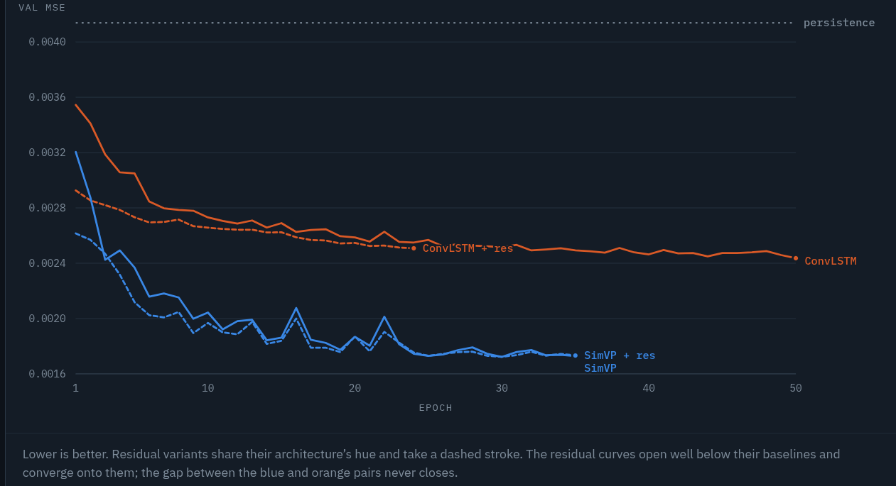
In our experiments we found out that they converged right where the bare models predicted. There was a head start because they were predicting essentially the last frame + delta but during the course of epochs, they converged to their predecessors.
We plan to implement and test more models and see which one performs best.
Configuration
Everything below was held identical across the four experiments, so the comparison is fair.
# data
T: 6                  # six past frames in, one frame out
crop_size: 256        # 256 x 256 tiles
crop_stride: 256      # non-overlapping, so 49 tiles per frame
target_channels: 1    # all 4 channels go in, only TIR1 comes out
splits:               # by date, with a buffer day between each
  train: 46 days
  val:    7 days
  test:   7 days      # sealed until a winner is picked

# training
loss: MSE             # mean squared error on normalised brightness temperature
optimizer: Adam
lr: 0.0001            # halved after 3 epochs with no improvement, floor 1e-6
epochs: 50            # but stop early after 10 epochs with no improvement
seed: 42              # same crops, same shuffle order, every run

# models
convlstm:             # 3 layers, 64 hidden channels, 3x3 kernels
  num_layers: 3
  hidden_dim: 64
  kernel_size: 3
  batch_size: 8
simvp:                # 64-channel encoder, 256-channel translator, 4 blocks each
  hid_S: 64
  hid_T: 256
  N_S: 4
  N_T: 4
  groups: 8
  batch_size: 24
The two batch sizes differ because ConvLSTM holds its hidden state at the full 256 x 256 resolution and simply will not fit 24 samples on a 24 GB card; SimVP does its work downsampled and will.
Results v1
Below is a simple summary of the main validation metrics:
| Model | Epochs | Val MSE | Skill | SSIM | PSNR | Training Time |
|---|---|---|---|---|---|---|
| SimVP | 30 | 0.001722 | 58.4% | 0.7894 | 27.639 | 23.2 h |
| SimVP + residual | 30 | 0.001723 | 58.4% | 0.7899 | 27.638 | 23.4 h |
| ConvLSTM | 50 | 0.002436 | 41.1% | 0.7475 | 26.134 | 46.2 h |
| ConvLSTM + residual (still training) | 25 | 0.002504 | 39.5% | 0.7425 | 26.014 | 23.7 h |
interesting problems
Before model training, there was a requirement to do preprocessing. Since the data is not that simple to understand, I may have made a couple of errors understanding it in the first few dry runs of models (lol).
First, the idea of lazy loading batches. In this project, we’re basically indexing using a manifest.json file. I didn’t know how that worked before this.
Some other few things to note:
- Fixed crop training - we fixed a 256 x 256 crop and decided we’ll train the models on this data. Result- we overfit that region. If you think that’s obvious, it is. In hindsight it is, but during my first try, I didn’t think about it and after training for 5-6 hours I realized the train loss just wouldn’t stop decreasing while the val loss stayed at 0.0102. Another question you could ask is, “how did you decide which region?” We checked for the most collective variance in a 256x256 crop in the WHOLE dataset and set that crop as the crop.
- training data - we first downloaded one month data to get the processing pipeline fixed. And using that we trained some models. Results were again bad because fixed crop size + less training data = overfit-maxxing
- How many channels do we use? - INSAT gave us 6. Initially we used one, to predict one. Now we’re using 4 channels, like we should have in the first place.
- GPUs?? - our beloved college let us use the HPC with the two beasts and we’ve been using them since. Be sure there were some issues to get this setup to work like how do we get the data up there? do we process here and then put the data or do we put raw data there? etc.
conclusion and future ideas
This is a very interesting project to me. I’ve finally figured out the pipeline. Using tools like Wandb, I now train models all day (literally, look at the training times of the models). What remains is training more models, trying different experiments and I’ll let you know when I have an update.
One would notice the blur prediction in the image of the start of the post. That’s a known issue of MSE based model trainings. It’s because the spatiotemporal movenment is averaged out by the criterion making it smoothen out the edges. There are ways to fix them. Which will be experimented with later.
Thank you for being here
~ Aayushya
References
- github for this project: https://github.com/aayushyatiwari/chase-the-cloud/tree/local
- mosdac website for data: https://mosdac.gov.in/uops/satellite
- Select INSAT 3DR as data source and category imager
- residual prediction idea: (paper link its idea was borrowed into video prediction tasks later by google)
- IMD paper : https://imetsociety.org/wp-content/pdf/vayumandal/2023491/2023491_5.pdf